R Code
On this page you will find R code for topics discussed in class.
Environmental Metrics at U-M
Here are data on environmental metrics for the University of Michigan. These data are published by the Office of Campus Sustainability.
The following code reads in the csv file and tidies the data for plotting. The dataset engy selects total energy consumption per person.
library(tidyverse)
library(stringr)

fin <- "FY2019 Env Metrics values - values.csv"
dat <- read_csv(fin, skip = 2)
head(dat)
## # A tibble: 6 x 17
## Energy FY2004 FY2005 FY2006 FY2007 FY2008 FY2009 FY2010 FY2011 FY2012
## <chr> <chr> <chr> <chr> <chr> <chr> <chr> <chr> <chr> <chr>
## 1 Total~ 6,624~ 6,370~ 6,855~ 6,330~ 6,338~ 6,509~ 6,903~ 7,168~ 7,414~
## 2 Total~ 91,11~ 86,26~ 91,24~ 83,12~ 81,17~ 82,21~ 85,72~ 87,92~ 89,25~
## 3 Total~ 3.22 3.03 3.19 2.71 2.6 2.62 2.52 2.55 2.51
## 4 Build~ 6,523~ 6,267~ 6,751~ 6,226~ 6,231~ 6,400~ 6,802~ 7,057~ 7,305~
## 5 Build~ 230,4~ 219,9~ 235,9~ 202,9~ 199,9~ 203,8~ 200,0~ 205,0~ 205,7~
## 6 Build~ 89,72~ 84,86~ 89,86~ 81,76~ 79,80~ 80,83~ 84,47~ 86,56~ 87,94~
## # ... with 7 more variables: FY2013 <chr>, FY2014 <chr>, FY2015 <chr>,
## # FY2016 <chr>, FY2017 <chr>, FY2018 <chr>, FY2019 <chr># Reshape the data into long form
dat <- dat %>%
gather(starts_with("FY"), key = "FY", value = "lvl")
head(dat)## # A tibble: 6 x 3
## Energy FY lvl
## <chr> <chr> <chr>
## 1 Total Energy Consumption (MMBtu) FY2004 6,624,545
## 2 Total Energy Consumption (Btu/person) FY2004 91,112,889
## 3 Total Energy Consumption (Btu/person/ft2) FY2004 3.22
## 4 Building Energy (MMBtu) FY2004 6,523,644
## 5 Building Energy (Btu/ft2) FY2004 230,487
## 6 Building Energy (Btu/person) FY2004 89,725,123dat <- dat %>%
mutate(year = as.numeric(str_sub(FY, start = 3, end = -1L)),
lvl = parse_number(lvl))## Warning: 3 parsing failures.
## row col expected actual
## 2833 -- a number Raw Data Overview
## 2884 -- a number Raw Data Overview
## 2940 -- a number Raw Data Overview# Grab energy consumption per person
engy <- filter(dat, Energy == "Total Energy Consumption (Btu/person)")
head(engy)## # A tibble: 6 x 4
## Energy FY lvl year
## <chr> <chr> <dbl> <dbl>
## 1 Total Energy Consumption (Btu/person) FY2004 91112889 2004
## 2 Total Energy Consumption (Btu/person) FY2005 86260879 2005
## 3 Total Energy Consumption (Btu/person) FY2006 91244604 2006
## 4 Total Energy Consumption (Btu/person) FY2007 83128476 2007
## 5 Total Energy Consumption (Btu/person) FY2008 81173920 2008
## 6 Total Energy Consumption (Btu/person) FY2009 82214756 2009Now we can plot the data. Here is total energy consumption per person at U-M:
# Total energy consumption per person
ggplot(data = engy) +
  geom_line(mapping = aes(x = year, y = lvl/1000000)) +
  labs(x = "Fiscal year", y = "Millions BTUs/person") +
  ggtitle("Total Energy Consumption")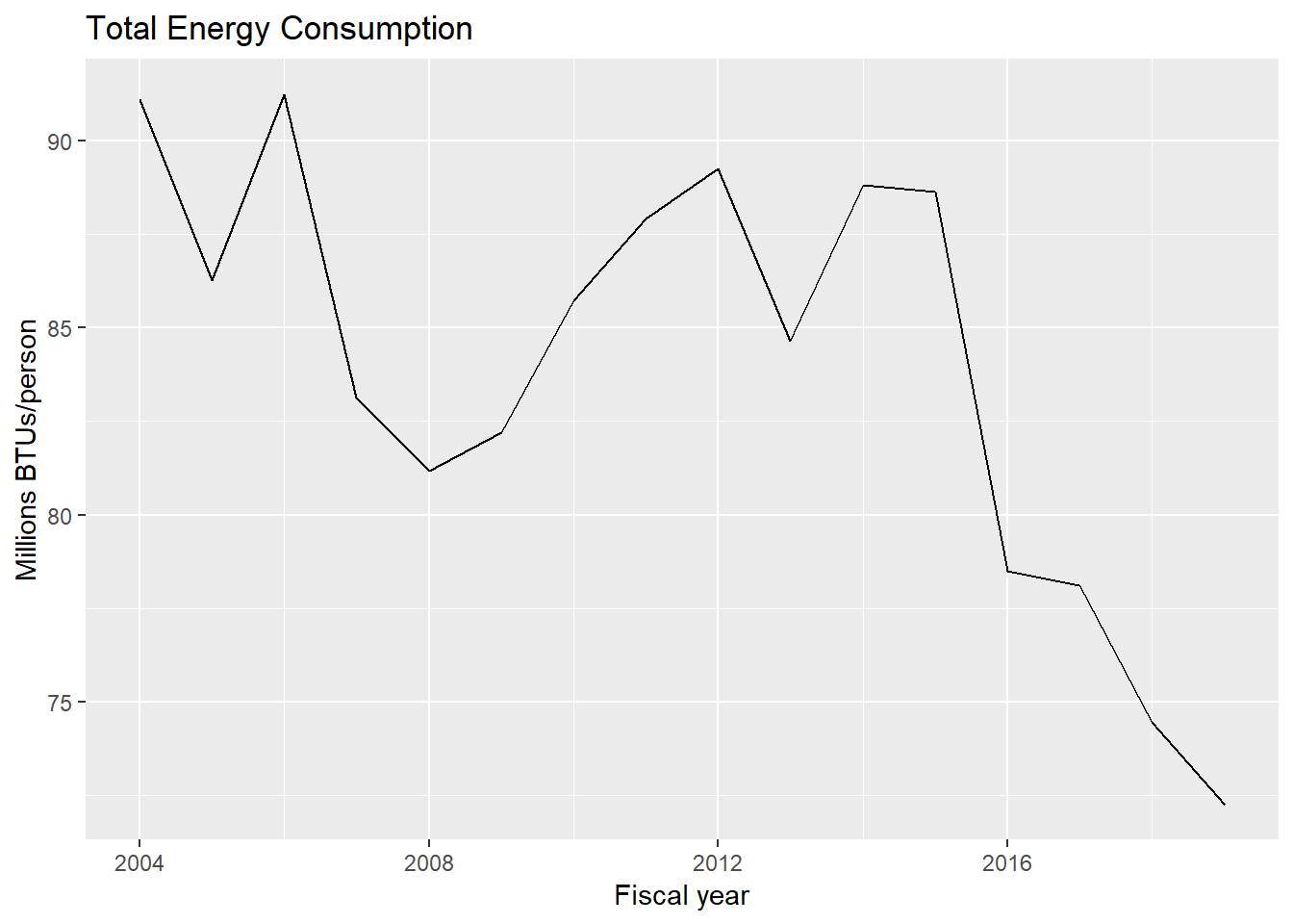
ggsave("fig-energy-C-per-person.png")
ggsave("fig-energy-C-per-person.eps")
Why is energy use per person falling after 2015? Is energy use going down? Or are there simply more people?
ggplot(data = filter(dat, Energy == "Total Campus Population")) +
  geom_line(mapping = aes(x = year, y = lvl)) +
  labs(x = "Fiscal year", y = "People") +
  ggtitle("Total Campus Population")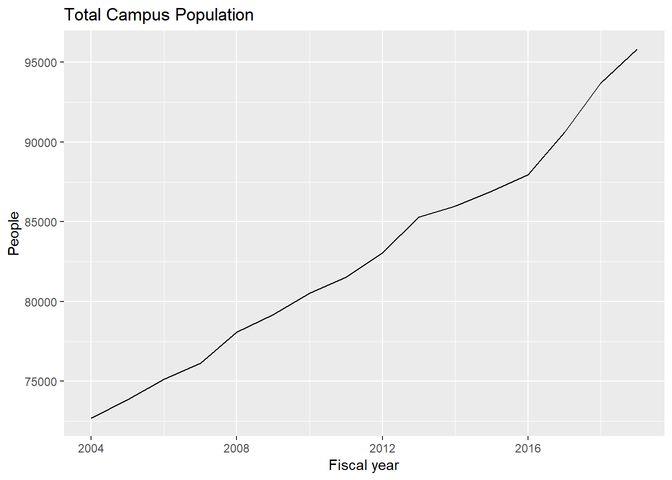
ggsave("fig-U-M-pop.png")
ggsave("fig-U-M-pop.eps")

ggplot(data = filter(dat, Energy == "Total Energy Consumption (MMBtu)")) +
  geom_line(mapping = aes(x = year, y = lvl)) +
  labs(x = "Fiscal year", y = "MMBTU") +
  ggtitle("Total Energy Consumption")
ggsave("fig-energy-C.png")
ggsave("fig-energy-C.eps")
Here is water use per person. The code grabs water use per person in the same step as generating the plot:
# Water use per person
ggplot(data = filter(dat, Energy == "Total Water Use (gal/person)")) +
  geom_line(mapping = aes(x = year, y = lvl/1000)) +
  labs(x = "Fiscal year", y = "Gallons/person (thousands)") +
  ggtitle("Total Water Use Per Person")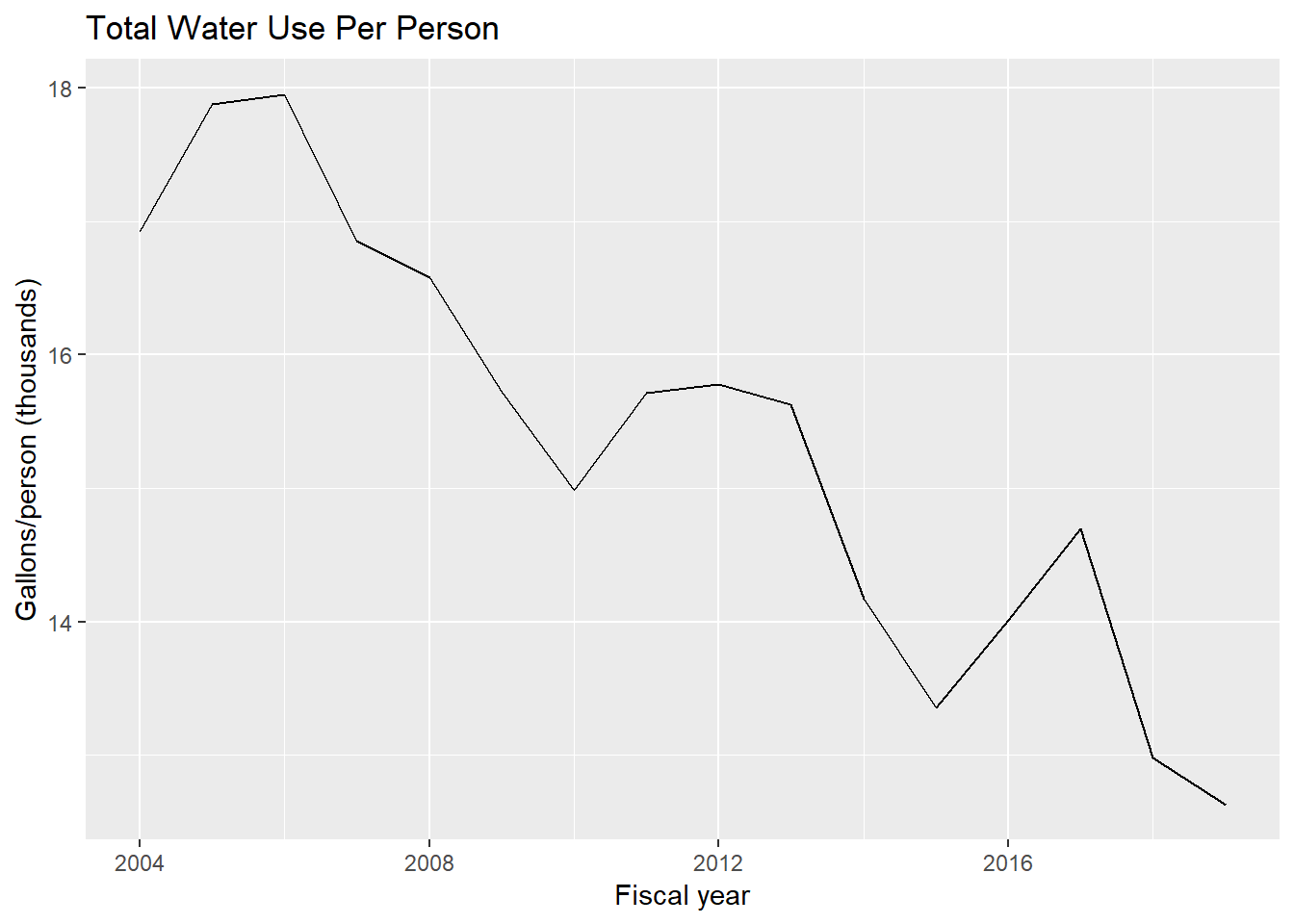
ggsave("fig-gallons-per-person.png")
ggsave("fig-gallons-per-person.eps")
Finally, this figure replicates the figure posted on the website—in maize and blue!
m_maize <- "#ffcb05"
m_blue <- "#00274c"
# Reproduce the figure from the website
ggplot(data = filter(dat, Energy == "Total Energy Consumption (MMBtu)")) +
  geom_col(mapping = aes(x = year, y = lvl/1000000, fill = "Trillions of BTUs")) +
  geom_line(data = filter(dat, Energy == "Total Energy Consumption (Btu/person/ft2)"),
            mapping = aes(x = year, y = lvl, color = "BTU per person per ft2"), size = 1.0) +
  labs(x = "Fiscal year", y = "") +
  scale_fill_manual(name = "", values = c("Trillions of BTUs" = m_blue)) +
  scale_color_manual(name = "", values = c("BTU per person per ft2" = m_maize)) +
  ggtitle("University of Michigan Total Energy Use")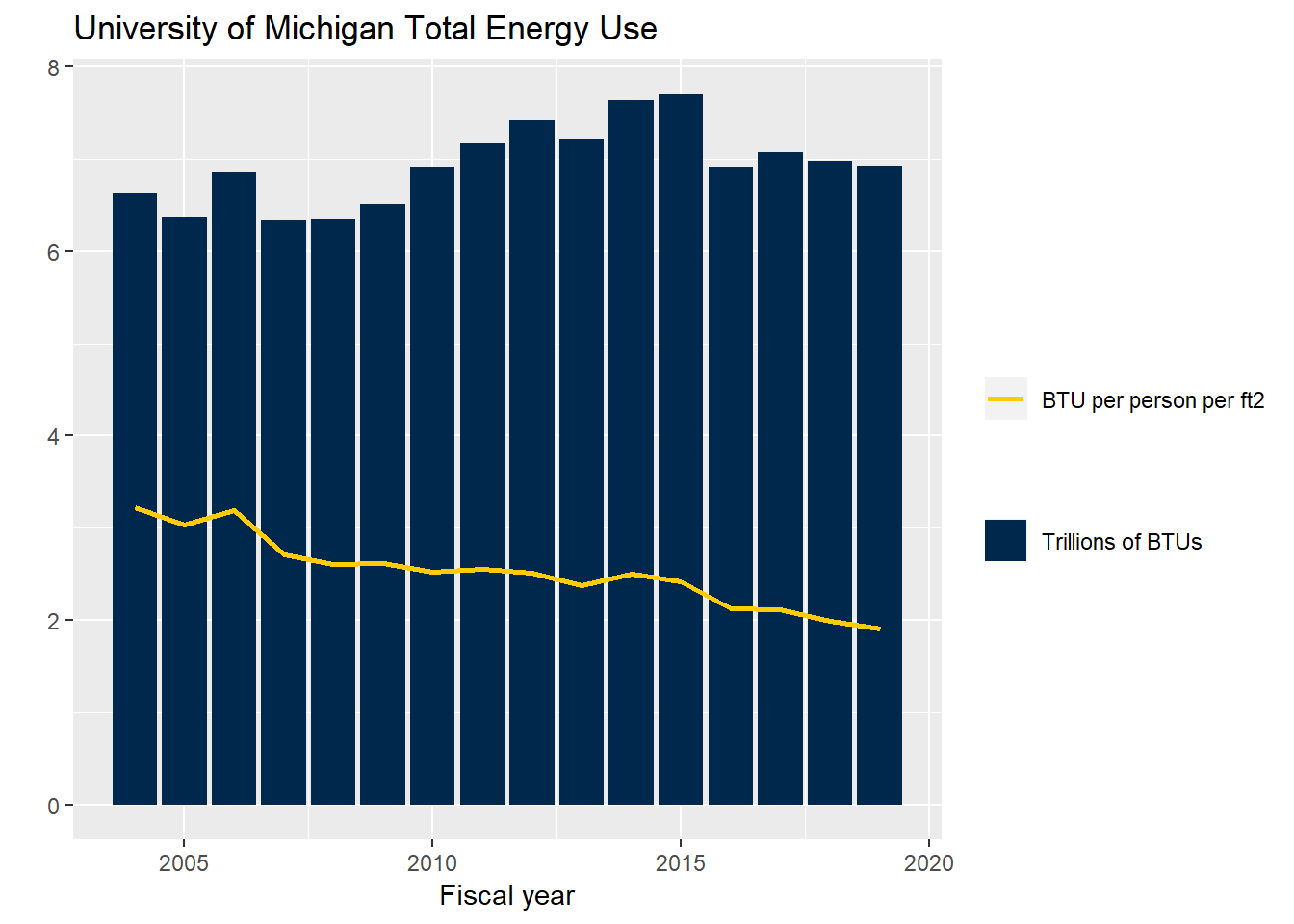
ggsave("fig-U-M-total-energy.png")
ggsave("fig-U-M-total-energy.eps")
Gamma Discounting
Here are the answers to the question
Taking all relevant considerations into account, what real interest rate do you think should be used to discount over time the (expected) benefits and (expected) costs of projects being proposed to mitigate the possible effects of global climate change?
Here are the raw data:
library(tidyverse)

rates <- c(1.0, 6.5, 6.0, 7.0, 2.0, 2.0, 2.0, 3.0, 1.0, 1.0, 3.0, 6.0, 0.5, 0.1, 2.0, 2.5,
          1.0, 1.0, 0.5, 1.8, 0.5, 1.0, 7.0, 5.0, 1.0, 4.0)

ggplot() +
  geom_histogram(mapping = aes(rates)) +
  labs(x = "Real discount rate (percent)", y = "Number of responses")
## `stat_bin()` using `bins = 30`. Pick better value with `binwidth`.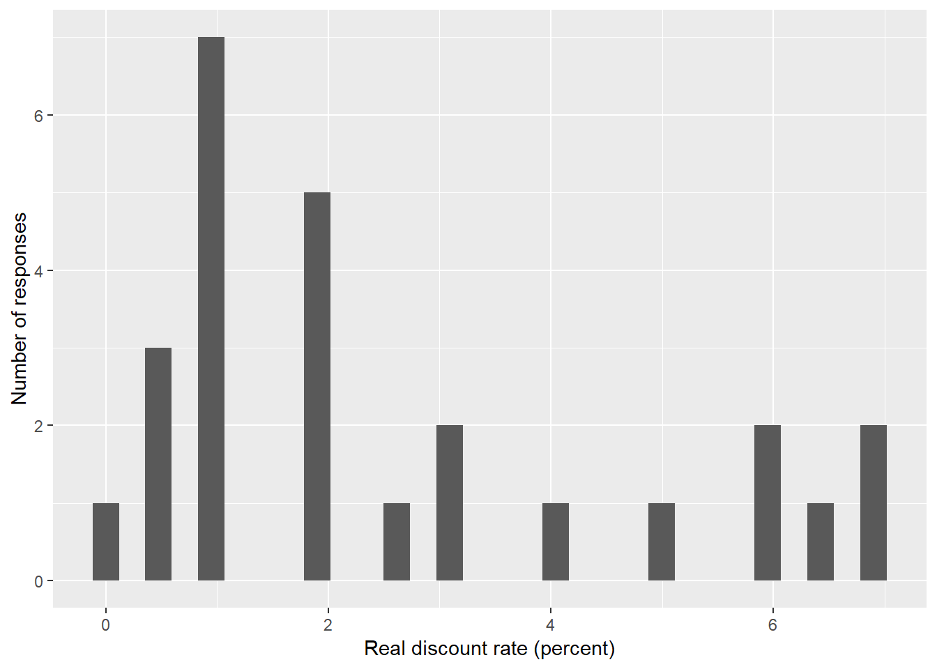
We can fit the data to a Gamma distribution. The command denscomp plots the histogram against fitted density function. What do you think?
fit_gamma <- fitdistrplus::fitdist(rates, distr = "gamma", method = "mle")
fitdistrplus::denscomp(fit_gamma, addlegend = FALSE, main = "",
                       xlab = "Real discount rate (percent)",
                       fitcol ="darkblue",
                       plotstyle = "ggplot")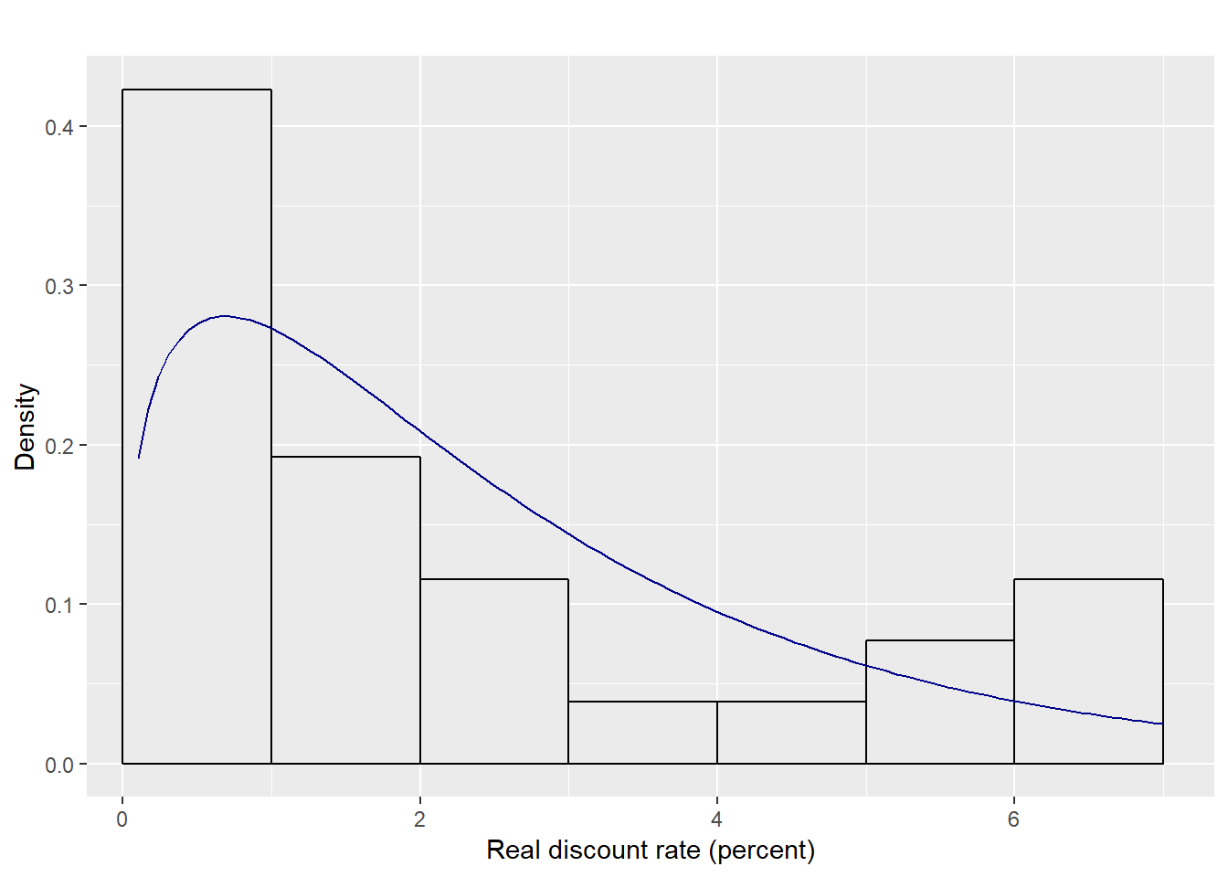
Google Trends: The Cost of Carbon
Here is code looks at the number of Google searches for “cost of carbon.” The search was motivated by our look at estimates of the social cost of carbon provided by Nordhaus (2017).
Descriptions of Google Trends data are provided at
The data on hits are indexed to 100, where 100 is the maximum search interest for the time and location selected. In our case, the location is all US states and the time is from 2004 onwards (until approximately 36 hours ago). To put the index into context, we are looking at patterns in the data through time.
For a comparison, I start by looking at the number of searches for global warming. The code defines search_terms and then searches for these terms using the R package gtrendsR. This R package retrieves and displays information provided by Google Trends.
To continually work on the website, I save the retrieved information to an rds file and comment out the code. You can simply uncomment the code to run your own query.
The index of hits is then plotted:
library(tidyverse)
library(tibble)
library(gtrendsR)
## Warning: package 'gtrendsR' was built under R version 3.6.1search_terms <- c("global warming")
# dat <- gtrends(keyword = search_terms,
# geo = "US",
# time = "all")
# (summary(dat))
#
# tsdat <- dat$interest_over_time
# # (glimpse(tsdat))
fdat <- "./dat_global_warming.rds"
# write_rds(tsdat, fdat)
tsdat <- read_rds(fdat)
ggplot(data = tsdat) +
geom_line(mapping = aes(x = date, y = hits), size = 0.9, color = "darkblue") +
labs(x = "", y = "Hits (index = 100 at maximum search interest)") +
ggtitle(str_to_title(search_terms))
Which is interesting—and not what I expected at all. I had guessed the time series would trend up through time. There appears to be a strong seasonal cycle.
scc_search_terms <- "social cost of carbon"Here is the trend in searching for social cost of carbon:
# scc <- gtrends(keyword = scc_search_terms,
#         geo = "US",
#         time = "all")
# (summary(scc))
#
# ts_scc <- scc$interest_over_time
# # (glimpse(ts_scc))
fdat_scc <- "./dat_scc.rds"
# write_rds(ts_scc, fdat_scc)
ts_scc <- read_rds(fdat_scc)

ggplot(data = ts_scc) +
  geom_line(mapping = aes(x = date, y = hits), size = 0.9, color = "darkblue") +
  labs(x = "", y = "Hits (index = 100 at maximum search interest)") +
  ggtitle(str_to_title(scc_search_terms))
Toxic 100
Origin story
Here is some R code that reads in the data on the “Top 100 Polluters.” The data are provided by The Political Economy Research Institute at the University of Massachusetts Amherst. The PERI data come from the Toxics Release Inventory in a user-friendly format.
The TRI are data collected from the US Environmental Protection Agency in accordance with the the Emergency Planning and Community Right-to-Know Act of 1986. According to the EPA’s website, the EPCRA “was passed in 1986 in response to concerns regarding the environmental and safety hazards posed by the storage and handling of toxic chemicals. These concerns were triggered by the 1984 disaster in Bhopal, India, caused by an accidental release of methylisocyanate. The release killed or severely injured more than 2000 people.” About six months later, “a similar incident occurred at the Institute, West Virginia.”
Part of the EPCRA’s Community Right-to-Know provisions include the TRI: “Facilities must complete and submit a toxic chemical release inventory form (Form R) annually. Form R must be submitted for each of the over 600 TRI chemicals that are manufactured or otherwise used above the applicable threshold quantities.”
Because the EPA’s TRI database can be hard to access, PERI provides the data in an accessible—sort of.
Do you get your electricity or gas from DTE?
R code for reading in the data
This R code loads in data for Toxic 100 Water Polluters Index. The toxic-hazard index is computed from pounds of water pollutants released directly to surface water plus estimated pounds released post-treatment multiplied by chemical-specific toxicity weights. The code computes the share of this index
Load R packages:
library(tidyverse) # R packages for data science
library(rvest)     # R package for scraping information from web pages
library(forcats)   # R package for working with factors
Read in the data using read_html from the rvest package:
toxic100_water <- read_html("https://grconnect.com/tox100wt/ry2017/index.php?search=top100&iframe=yes")
tbl <- html_nodes(toxic100_water, "table") %>%
  html_table(fill = TRUE, header = TRUE) %>%
  .[[1]]

# Convert the dataset to a tibble, a fundamental part of the tidyverse
dat <- as_tibble(tbl)
head(dat)
## # A tibble: 6 x 7
## `Toxic 100 Wate~ Corporation `Toxic hazard (~ `Millions of po~
## <int> <chr> <chr> <chr>
## 1 1 DowDuPont 63,470,403,546 3.02
## 2 2 Northrop G~ 37,651,979,847 <0.01
## 3 3 Parker-Han~ 22,284,466,197 <0.01
## 4 4 Honeywell ~ 6,001,188,020 0.10
## 5 5 Southern C~ 3,086,597,686 0.09
## 6 6 DTE Energy 3,029,107,094 0.04
## # ... with 3 more variables: `Millions of pounds discharged to public
## # sewage treatment works` <chr>, `Millions of pounds of toxic
## # post-treatment releases` <chr>, `% of toxic hazard from a single
## # facility` <chr>tail(dat)## # A tibble: 6 x 7
## `Toxic 100 Wate~ Corporation `Toxic hazard (~ `Millions of po~
## <int> <chr> <chr> <chr>
## 1 95 Panasonic 19,119,135 <0.01
## 2 96 Procter & ~ 18,787,863 <0.01
## 3 97 Cabot 17,883,461 <0.01
## 4 98 Caterpillar 17,615,831 <0.01
## 5 99 Entergy 17,178,494 <0.01
## 6 100 Snap-on 16,033,523 ""
## # ... with 3 more variables: `Millions of pounds discharged to public
## # sewage treatment works` <chr>, `Millions of pounds of toxic
## # post-treatment releases` <chr>, `% of toxic hazard from a single
## # facility` <chr>Convert the toxic hazard, which is currently a string, into a number:
dat <- dat %>%
  mutate(haz = as.numeric(str_replace_all(`Toxic hazard (pounds released x toxicity)`, ",", "")))
The data are already arranged by toxic harzard, but we can double-check:
library(dplyr)
dat <- dat %>%
  arrange(-haz) %>%
  mutate(check_rank = row_number())
(select(dat, check_rank, `Toxic 100 Water Rank`))
## # A tibble: 101 x 2
## check_rank `Toxic 100 Water Rank`
## <int> <int>
## 1 1 1
## 2 2 2
## 3 3 3
## 4 4 4
## 5 5 5
## 6 6 6
## 7 7 7
## 8 8 8
## 9 9 9
## 10 10 10
## # ... with 91 more rowsNote: The check is not the same as the original rank because mysteriously there are two companies ranked 94. Your guess here is as good as mine.
Now we can compute the average index score for each company, mean(haz), and then compute how much each company’s index is relative to the average, haz/mean(haz) - 1 = ((haz) - mean(haz)) / (mean(haz)):
dat <- dat %>%
  mutate(haz_rel = 100*(haz / mean(haz) - 1))
Let’s plot the shares of the first 10 companies:
dat10 <- filter(dat, `Toxic 100 Water Rank` <= 10) %>%
  mutate(Corporation = factor(Corporation))

ggplot(data = dat10) +
  geom_point(mapping = aes(x = haz_rel, y = fct_reorder(Corporation, haz_rel))) +
  labs(x = "Percent larger than the average among Top 100", y = "") +
  ggtitle("Toxic 100 Water Polluters")
DowDuPont’s toxic-hazard index is over 3,000 times the average index in the Toxic 100 Water Polluters list. DTE’s index is 78 times the average. BASF’s index is 13.6 times the average.
The graph shows that water pollution is concentrated among a few emitters.
Finally, here’s a csv file of the data for you to download:
dat <- dat %>%
  select(-check_rank)
write_csv(dat, "toxic100_water.csv")
The csv file is available to download here.
Resources
I used a few sources when trying to figure out how to read the data:
- This blog post on scraping HTML table
- The queries used seem to come from this website.
- Project-oriented workflow by Jenny Bryan
Pollution abatement
Introduction
Tietenberg and Lewis (2018) always offer a powerful quote at the begining of a chapter. They offer this quote from Charles Yost at the begining of chapter 14, “Economics of Pollution Control”:
Deomocracy is not a matter of sentiment, but of foresight. Any system that doesn’t take the long run into account will burn itself out in the short run.
The burn-itself-out part of the quote likely refers to global warming, emphasizing the stakes. Action taken to prevent global warming includes carbon regulation. This note covers three examples of carbon regulation.
The first is a command-and-control approach. Under command and control, the government specifies the policy instrument. Emissions standards are an example of the command-and-control approach. The second is a tax emitted on each unit of emmssion. The third is a cap-and-trade system. Under a cap-and-trade system, there is a collective emissions limit and each firm is allocated allowances to emit. The allowances add up to the emmissions limit. The allocation of allowances among firms is done in many ways. For example, the government can endow firms with allowances or have firms bid on allowances in an auction.
Technology of polluation abatement
Each firm has access to technologies capable of reducing emmissions. These technologies are high-tech smokestack scrubbers (HTSS), low-tech smokestack scrubbers (LTSS), upgrades to boilers, upgrades to generators, switch fuel to coal/oil blend, and purchases or sales of credits. Technologies differ in the amount they reduce emmissions and their cost for each firm.
The technologies are listed in the table below:
| Technology | Giant | Detroit | Coalcoa | Ontario | Fossil | Quebec |
|---|---|---|---|---|---|---|
| HTSS | 2.5 | 2.5 | 2.5 | 2.5 | 1 | 1.5 |
| LTSS | 2 | 2 | 2 | 2 | 1 | NA |
| Upgrade Boilers | 1 | 1 | 0.5 | 1 | 1 | 1 |
| Upgrade Generators | 1 | 1 | 1 | 0.5 | 0.5 | 0.5 |
| Switch to Gas | 0.5 | 0.5 | 1 | 1 | 0.5 | 0.5 |
The Detroit company, for instance, can upgrade their boilers and lower emissions by 1 metric ton per year.
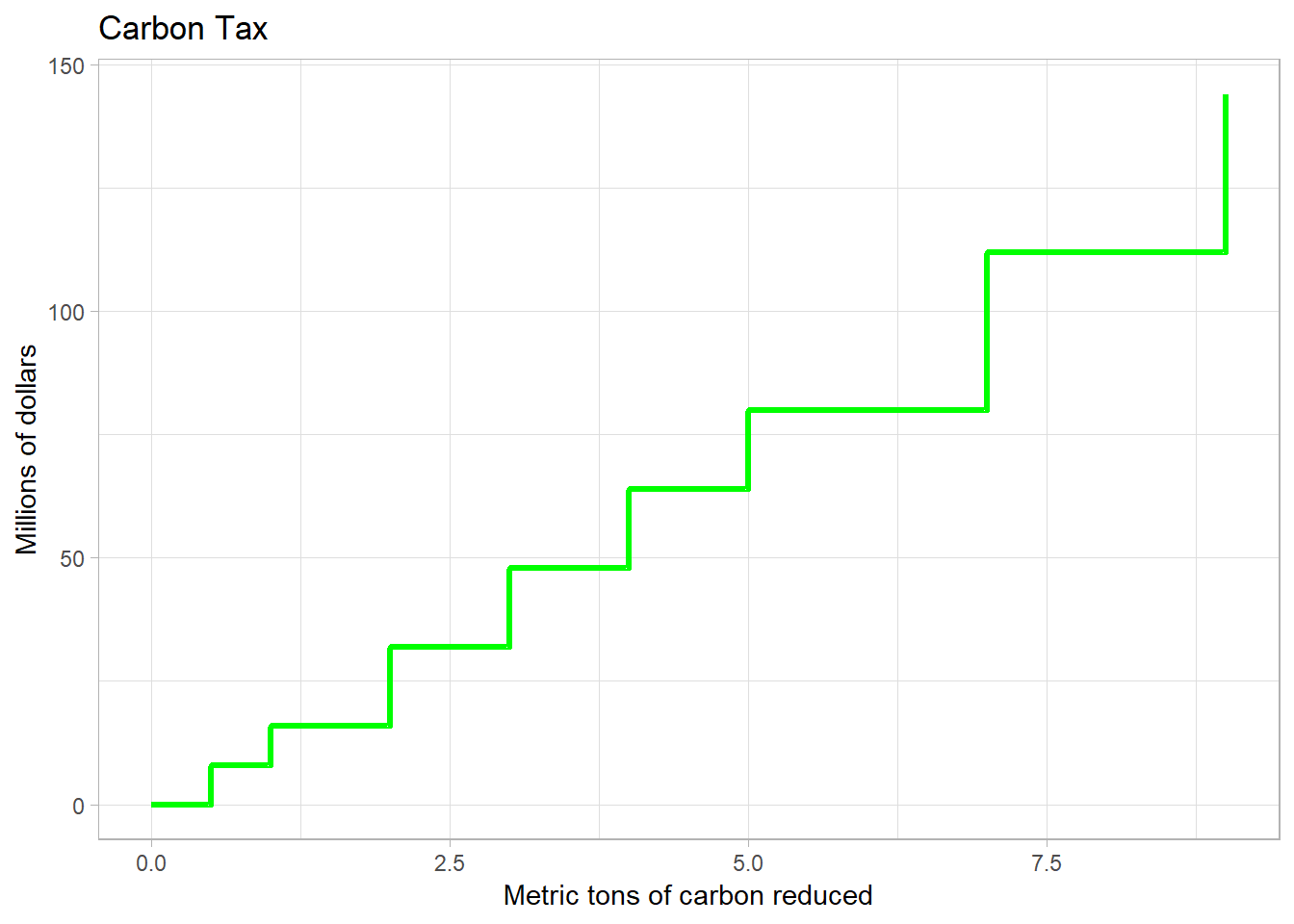
Command and control
The first policy instrument considered is command and control. Under command and control, the government specifies the policy instrument. For us, the policy instrument specified is the installation of high-tech scrubbers.
The below table lists the cost per metric ton of annual reductions by firm. From the table, the least expensive way to reduce carbon emmissions by one ton is for Giant or Detroit to install high-tech scrubbers
| Technology | Firm | Reduction | Cost | Cost/Ton |
|---|---|---|---|---|
| HTSS | Giant | 2.5 | 60 | 24 |
| HTSS | Detroit | 2.5 | 60 | 24 |
| HTSS | Coalcoa | 2.5 | 65 | 26 |
| HTSS | Ontario | 2.5 | 80 | 32 |
| HTSS | Quebec | 1.5 | 50 | 33.33 |
| HTSS | Fossil | 1 | 60 | 60 |

The above figure depicts the cost of reducing carbon if installation of high-tech scrubbers are installed according to cost per ton. (Note: This isn’t the cost-minimization solution—but is a close rule of thumb.) From the table, Giant install HTSS and 2.5 metric tons of carbon are reduced. This reduction costs 60 million dollars. Next Detroit install HTSS, reducing carbon by another 2.5 metric tons at a cost of 60 million. At this point 5 metric tons of carbon have been reduced for a total cost of 120 million. This point is indicated by the black dot in the figure.
The remainder of the figure is generated by similarly cumulating carbon reduction and costs.
Carbon Tax
The carbon tax charges 20 million dollars for every ton of carbon emitted. All firms have the option of installing technology to reduce emmissions. How does each firm choose what technologies to install?
Consider Detroit. Detroit can either install technologies or pay 20 million per every ton of carbon emitted. Looking at the table below, Detroit can pay 60 million to install HTSS, but this costs 24 million per ton. Better to pay the tax than install HTSS.
What about LTSS? In this case, Detroit can pay 32 million to install LTSS and reduce carbon by 2 units. Under the tax, those 2 units would cost 40 million. Better to install LTSS.
For a decision rule, Detroit looks at the marginal cost of reducing a unit of emmissions. If that cost is below 20, Detroit chooses to install the reduction technology. Looking at the table, Detroit install all technologies except HTSS.
| Technology | Reduction | Cost | Marginal cost |
|---|---|---|---|
| HTSS | 2.5 | 60 | 24 |
| LTSS | 2 | 32 | 16 |
| Upgrade Boilers | 1 | 16 | 16 |
| Upgrade Generators | 1 | 16 | 16 |
| Switch to Gas | 0.5 | 8 | 16 |
The below figure depicts the cost of reductions under the carbon-tax policy instrument. The figure reflects the same ordering procedure used to create the command-and-control figure.
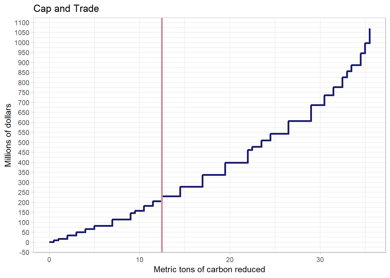
Cap and Trade
What happened under the carbon-tax policy instrument? Imagine there are two firms. Each firm has access to a technology that reduces emmissions. The costs of reduction for firms \(1\) and \(2\) are \(c_1(r_1)\) and \(c_2(r_2)\), where \(r_1\) and \(r_2\) are the amounts of reduction done at the two firms.
The problem of minimizing the cost of reducing pollution to \(\bar{r}\) can be written \[\begin{align*} \min_{r_1,r_2} c_1 \left( r_1 \right) + c_2 \left( r_2 \right) \end{align*} \] subject to \[\begin{align*} r_1 + r_2 = \bar{r}. \end{align*} \]
We can substitute the constraint into the objective by noting that \(r_2 = \bar{r} - r_1\). Because \(\bar{r}\) is given, choosing \(r_1\) provides a choice of \(r_2\) through the constraint. Using this substitution, the problem becomes \[\begin{align*} \min_{r_1} c_1 \left( r_1 \right) + c_2 \left( \bar{r} - r_1 \right). \end{align*} \] The associated first-order condition for \(r_1\) is \[\begin{align*} \text{mc}_1 \left( r_1 \right) - \text{mc}_2 \left( \bar{r} - r_1 \right) = 0. \end{align*} \] Re-arranging yields \[\begin{align*} \text{mc}_1 \left( r_1 \right) = \text{mc}_2 \left( r_2 \right), \end{align*} \] where we’ve used that fact that \(r_2 = \bar{r} - r_1\). The cost-minimizing solution, in other words, has firms equalizing marginal cost.
Imagine if this wasn’t the case. It would be possible to lower costs by having the high-marginal-cost firm reduce their reduction by \(1\) and have the low-marginal-cost firm increase their production by \(1\). Total reductions would be the same, but costs would be less.
Remarkably this was nearly the solution under the tax system. All firms were checking whether their marginal costs were equal to \(20\). This reasoning suggests that using a tax as a policy instrument reduces costs when trying to reach a reduction target like \(\bar{r}\).
The cap-and-trade system has similar incentives. Imagine if the two firms are are endowed with rights rights to pollute, like they are here. A firm has to reduce pollution if its allowance is below the pollution cap. The high-marginal-cost firm in this scenario will be willing to buy from the low-marginal-cost firm. The low-marginal-cost firm can reduce its pollution and sell their reduction to the high-marginal-cost firm. The end result is the tax solution.
The cap-and-trade system also minimizes costs. The below figure depicts the costs for reducing emmissions where technologies are implemented according to cost per ton.
There are five firms. Each is endowed with the right to emit 7.5 tons of carbon and each needs to reduce emmissions by 2.5. Total reduction needs to be 12.5. Total costs should be around 225 million.
The next section compares the three systems.
Comparison of all three systems
The below figure depicts the costs of reduction for the command-and-control, tax, and cap-and-trade policy instruments. The command-and-control system costs the most. For a given amount of reduction, this policy instrument costs most. The carbon tax and cap-and-trade system both minimize costs for a given amount of reduction. This is seen in the figure by the overlap of the green and yellow lines.
Whether or not the cap-and-trade policy instrument produces low costs in practice depends on trading frictions. We’ll have to see how it plays out.

References
Nordhaus, William D. 2017. “Revisiting the Social Cost of Carbon.” Proceedings of the National Academy of Sciences 114 (7): 1518–23. https://doi.org/10.1073/pnas.1609244114.
Tietenberg, Tom, and Lynne Lewis. 2018. Environmental and Natural Resource Economics. 11th ed. New York, NY: Routledge.