Welcome to my professional website!

I made the devastating choice of updating Hugo and blogdown, which required a major revamp of my professional website This blog post by Alison Hill was useful for learning about the latest version of blogdown.

Below is documentation for writing Markdown.

Math

Including \(\LaTeX\) is straightforward: When \(a \ne 0\), there are two solutions to \(ax^2 + bx + c = 0\) and they are $$x = {-b \pm \sqrt{b^2-4ac} \over 2a}.$$

Example math block:

\begin{align*} \gamma_{n} = \frac{ \left | \left (\mathbf x_{n} - \mathbf x_{n-1} \right )^T \left [\nabla F (\mathbf x_{n}) - \nabla F (\mathbf x_{n-1}) \right ] \right |}{\left \|\nabla F(\mathbf{x}_{n}) - \nabla F(\mathbf{x}_{n-1}) \right \|^2} \end{align*}

R

Here is R code that runs a linear regression:

summary(cars)
##      speed           dist       
##  Min.   : 4.0   Min.   :  2.00  
##  1st Qu.:12.0   1st Qu.: 26.00  
##  Median :15.0   Median : 36.00  
##  Mean   :15.4   Mean   : 42.98  
##  3rd Qu.:19.0   3rd Qu.: 56.00  
##  Max.   :25.0   Max.   :120.00
fit <- lm(dist ~ speed, data = cars)
summary(fit)
## 
## Call:
## lm(formula = dist ~ speed, data = cars)
## 
## Residuals:
##     Min      1Q  Median      3Q     Max 
## -29.069  -9.525  -2.272   9.215  43.201 
## 
## Coefficients:
##             Estimate Std. Error t value Pr(>|t|)    
## (Intercept) -17.5791     6.7584  -2.601   0.0123 *  
## speed         3.9324     0.4155   9.464 1.49e-12 ***
## ---
## Signif. codes:  0 '***' 0.001 '**' 0.01 '*' 0.05 '.' 0.1 ' ' 1
## 
## Residual standard error: 15.38 on 48 degrees of freedom
## Multiple R-squared:  0.6511,	Adjusted R-squared:  0.6438 
## F-statistic: 89.57 on 1 and 48 DF,  p-value: 1.49e-12

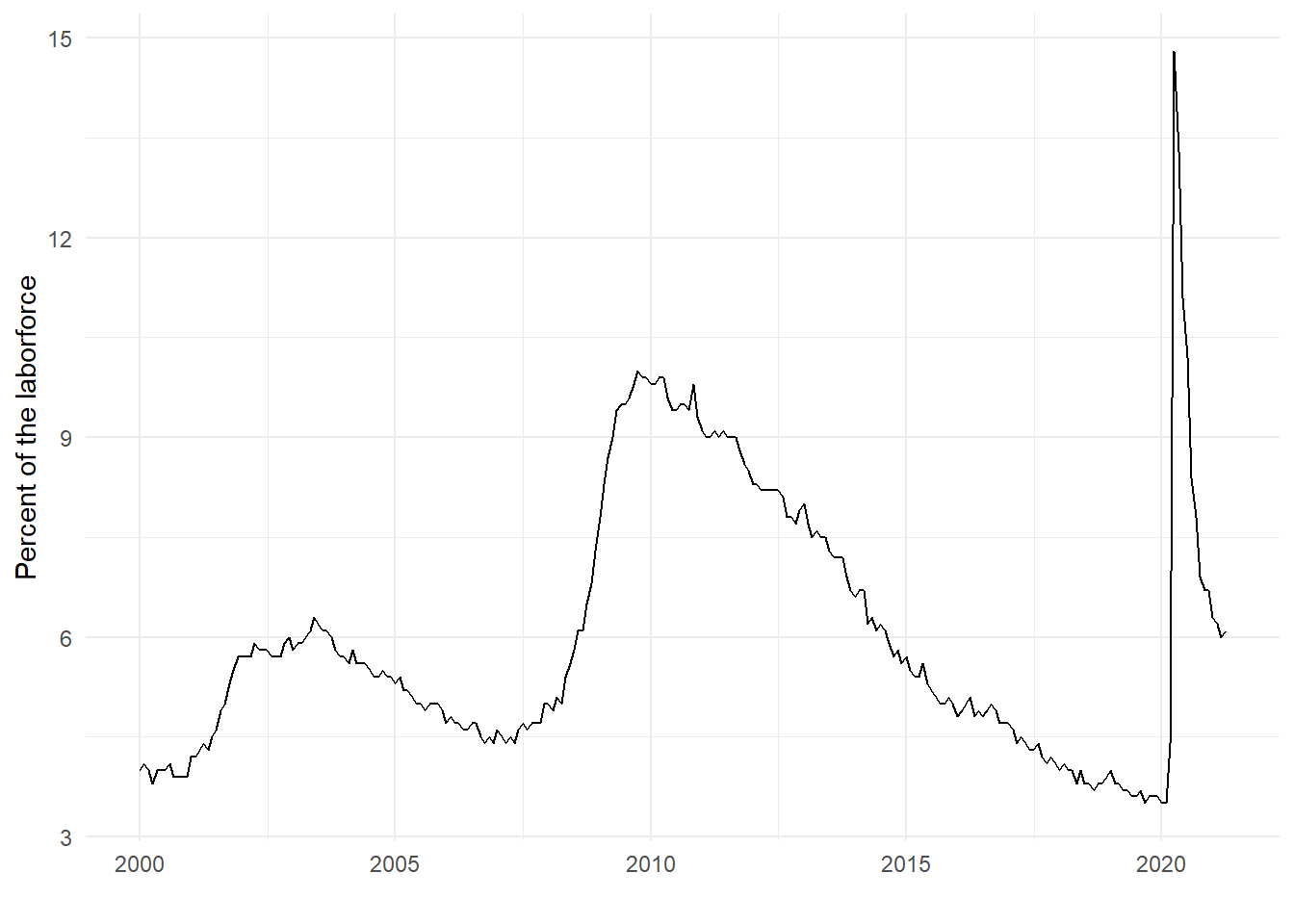
And here is R code that plots figure 1:

library(ggplot2)
library(tidyquant)
## Loading required package: lubridate
## 
## Attaching package: 'lubridate'
## The following objects are masked from 'package:base':
## 
##     date, intersect, setdiff, union
## Loading required package: PerformanceAnalytics
## Loading required package: xts
## Loading required package: zoo
## 
## Attaching package: 'zoo'
## The following objects are masked from 'package:base':
## 
##     as.Date, as.Date.numeric
## 
## Attaching package: 'PerformanceAnalytics'
## The following object is masked from 'package:graphics':
## 
##     legend
## Loading required package: quantmod
## Loading required package: TTR
## Registered S3 method overwritten by 'quantmod':
##   method            from
##   as.zoo.data.frame zoo
## == Need to Learn tidyquant? ====================================================
## Business Science offers a 1-hour course - Learning Lab #9: Performance Analysis & Portfolio Optimization with tidyquant!
## </> Learn more at: https://university.business-science.io/p/learning-labs-pro </>
dat <- tq_get("UNRATE", get = "economic.data", from = "2000-01-01")

ggplot(data = dat) +
  geom_line(mapping = aes(x = date, y = price)) +
  labs(x = "", y = "Percent of the laborforce") +
  theme_minimal()

Figure 1: Unemployment rate from 2000 onwards, monthly.